

Optimizing business workflows with custom Google Sheets solutions - Streamlining operations - Automating processes - Building dynamic dashboards 👇👇👇
Book a free call 👉
Joined June 2024
- Tweets1.5K
- Following235
- Followers371
- Likes3K





Google Sheets just got even faster! 🔥
Yesterday they did performance upgrades:
✅ 50% faster pasting from another sheet
✅ 50% faster filter conditions
✅ 30% faster loading of existing data
Anyone noticed the difference?
3
11
479
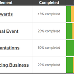
"I am looking for a progress bar within a cell, where the colors indicate the metric performance."
The formula SPARKLINE will assist you 🤗
=SPARKLINE(
{COUNTIF(Awards!F3:F,"Completed"),
COUNTIF(Awards!F3:F,"Work In Progress"),
COUNTIF(Awards!F3:F,"Not Started")},
{"charttype", "bar";
"color1", "#3aad1c";
"color2", "#ffc041";
"color3", "#ff4141"})
The first COUNTIF listed is allocated to color1. The second COUNTIF is allocated to color2. The order updates chronologically.
To customize the color of that progress bar, go to the paint bucket in the toolbar. Select the color you would like. Copy the Hex code and paste it into the formula.

2
11
512

Learn from my Google Sheets panic moment today... 😅
Ever seen this error? 👉 "PIVOT evaluates to an out-of-bounds range"
Here is what happened:
I set up pivot tables to function as scorecards, making my data slicer update them immediately (perfect for a dynamic dashboard) 🚀
But I made a mistake....
My pivot table range was A:D
My data slicer was referencing A:I
This mismatch triggered the error when I started to test it.
The fix? Adjust the pivot table range to match the slicers.
Have you encountered this error before?

2
6
397
I keep waking up, filled with such gratitude!
✨I have internal peace.
✨I have great health.
✨I have the sun pouring through the window.
✨I have goals that align with my belief system.
✨I have the opportunity to make decisions for my business.
✨I have work I am dying to finish to track the impact.
✨I have an amazing network of like-minded people.
✨I have uplifting friends and family
I have the present moment!
It is a huge juxtaposition to last year; being in this position today is such a special gift! 😁✨
No matter the season I have been in, I always do my daily gratitude for my first cup of coffee. My version of "smelling the roses". When I get out of bed, I put one foot down "Thank" and then, the other foot down "You".
What are you grateful for today?
Is your business growing but your processes are not?
Try Google Sheets paired with Google Apps Script to:
✅ Automate repetitive tasks
✅ Streamline workflows
✅ Deploy solutions tailored to your needs
1
8
401
The Ultimate Data Party 🎉
=TEXTJOIN(delimiter, TRUE, text1, text2, ...)
Like bringing together all your favorite party guests 🔢🔤
2
12
289
This is a great case study to show the true power of Google Sheets 🚀
From route planning, invoicing, databases and reporting, you cannot go wrong with a platform that is free, while being data-encrypted.

This is how to take INSPIRATION:
He found some LCVs (tempos) EMPTY, so he thought why not use them?
So he QUIT his job to run the UBER of LCVs from a GOOGLE SHEET.
... which now makes 2700 CRORES in REVENUE:
Here's the MIND BLOWING STORY behind Porter:

2
8
360
Concatenate Like a Cat on a Keyboard 🐾⌨️
=CONCATENATE(cell, another cell, another other cell, ....)
5
193
Smarten up your Summing 🧮
=SUMIFS(data range you want to sum,
first range you want to filter on, first range criteria,
second range you want to filter on, second range criteria,...)
Get exactly the total you need without the headache of manual calculations.
1
4
181
Book a call with me if you want smart sheets: calendly.com/kathryn-rose-be…
1
143
Dump Data with Ease 💥
=IMPORTRANGE("spreadsheet url", "Sheet!Data Range")
It pulls data from another sheet without the painful manual copying & pasting every time there is a change.
Because, let's be real.... copy & paste is 💩
1
6
199
Sorting without sorting! 🧠
Leave the manual sorting behind.....
=SORT(range, number of that column you want sorted, TRUE (ascending) or FALSE (descending))
Now you have sorted data in a new spot, without touching your original dataset 🎉
4
195
Let TRANSPOSE handle it for you 🔄
Need to swap rows into columns?
=TRANSPOSE(range)
No manual edits & no copy-pasting nightmares 🎭
4
139
Getting the logic right in a formula can be a challenge.
Here is your reminder: you do not have to solve it all in one go or in a single cell 😊 break it down into smaller steps across multiple columns. Give yourself time to think it through, and when it all makes sense, combine it into one formula 👍

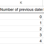
Today, I could not obtain the correct formula to list previous mileage per vehicle in date order. This information is essential for calculating the distance driven per tank and determining various metrics.
Here was my final formula:
=IFERROR(MAX(FILTER(D:D, B:B=B2, A:A<A2)), "")
Here is the logic in words:
=IFERROR(MAX(FILTER(Mileage, Vehicle License Plates=Current Record License Plate, Date < Current Record Date)), "")
How do you solve things in Google Sheets when you cannot get the logic to work? 🤔

Why Google Sheets? 😕
G - Great real-time colab
O - Optimizing workflows
O - Optimal and adaptable
G - Grows with your needs
L - Lightweight and simple
E - Easy, intuitive interface
S - Seamlessly integrates
H - Highly customizable
E - Efficient in handling data
E - Enables access anywhere
T - Thousands of templates
S - Secure and data-encrypted
A simple formula to extract the first letter and create an acrostic:
=LEFT(A1, 1) & " - " & A1
If you need some formatting:
=UPPER(LEFT(A1, 1)) & " - " & UPPER(LEFT(A1, 1)) & LOWER(MID(A1,2,999))
(one of my favorite techniques in cleaning up data😁)
1
2
97
Book a call with me if you need help with automating data cleaning processes calendly.com/kathryn-rose-be…
2
82